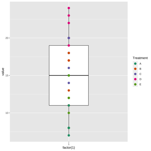
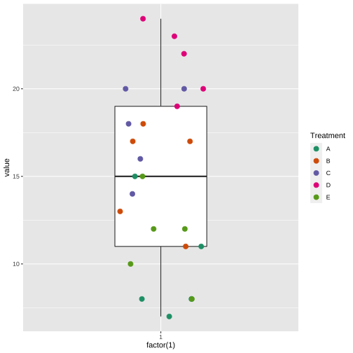
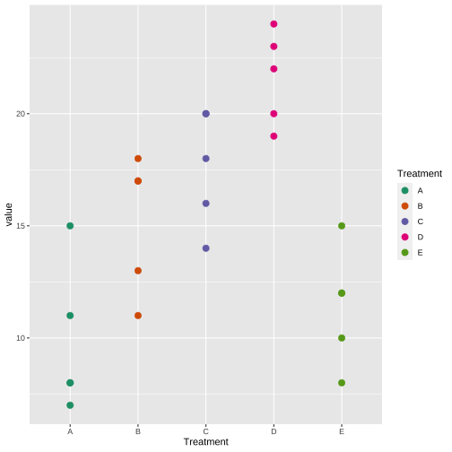
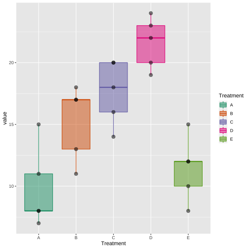
STA 225 2.0 Design and Analysis of Experiments

class: center, middle, inverse, title-slide

# STA 225 2.0 Design and Analysis of Experiments
## Lecture 3
### Dr Thiyanga S. Talagala
### 2021-10-29

---

<style>

.center2 {
  margin: 0;
  position: absolute;
  top: 50%;
  left: 50%;
  -ms-transform: translate(-50%, -50%);
  transform: translate(-50%, -50%);
}

</style>

## Completely Randomized Design (CRD)

- The simplest experimental design - CRD

- The treatments are assigned completely at random so that each experimental unit has the same chance of receiving every treatment.

- Appropirate only for experiments with **homogeneous** experimental units

---

## Example

**Objective of the study:** Effect of fertilizer dose on the yield of chille

**Experimental design:** CRD

**Independent variable:** Fertilizer doses

**Treatment:** Different doses of fertilizer (A, B, C, D, E)

**Dependent variables:** Number of chilles after one month

**Number of replicates:** 5

**Number of experimental units:** `$\sum_{i=1}^{t}r_i = 25$`, where `$t$` is the number of treatments ( `$t = 1, 2, 3, 4, 5$` ) and `$r_i$` number of replicates under treatment `$i$`

---

## Step 1: Assign treatments at random

---

## Step 2: Measure the response variable

---
## Step 3: Organize data

---

## Step 4: Exploratory data analysis

.pull-left[

![](L3_DOE_files/figure-html/unnamed-chunk-2-1.png)

]

.pull-right[

![](L3_DOE_files/figure-html/unnamed-chunk-3-1.png)

]

---

## Step 4: Exploratory data analysis

.pull-left[

![](L3_DOE_files/figure-html/unnamed-chunk-4-1.png)

]

.pull-right[

![](L3_DOE_files/figure-html/unnamed-chunk-5-1.png)

]

---

.pull-left[

```r
library(tidyverse)
A <- c(8, 8, 15, 11, 7)
B <- c(11, 17, 13, 18, 17)
C <- c(14, 16, 18, 20, 20)
D <- c(20, 24, 22, 19, 23)
E <- c(8, 10, 12, 15, 12)
df <- data.frame(A=A, B=B, C=C, D=D, E=E)
df <- df %>% pivot_longer(1:5, "Treatment", "value")
df$Treatment <- as.factor(df$Treatment)
df %>% group_by(Treatment) %>% summarise(
    mean=mean(value),
    sd=sd(value),
    median=median(value),
    min=min(value),
    max=max(value))
```

```
# A tibble: 5 × 6
  Treatment  mean    sd median   min   max
  <fct>     <dbl> <dbl>  <dbl> <dbl> <dbl>
1 A           9.8  3.27      8     7    15
2 B          15.2  3.03     17    11    18
3 C          17.6  2.61     18    14    20
4 D          21.6  2.07     22    19    24
5 E          11.4  2.61     12     8    15
```

]

.pull-right[

![](L3_DOE_files/figure-html/unnamed-chunk-7-1.png)

]

---

## Sources of Variation

- Source of variation due to **treatments**

- Source of variation due to **experimental error**

## Partition of total variability

<div class = "red">
`$$\textbf{Variability}_\text{total} = \textbf{Variability}_\text{treatment} + \textbf{Variability}_\text{experimental error}$$`
</div>

---

## Notations

| Treatment (level) 	|  R1 	|  R2	|  ...	| Rn 	| Totals 	|  Averages	|
|:---:	| :-----:	| :---:	| :---:	| :---:	| :---:	| :---:	|
|  1	| `$y_{11}$` 	|  `$y_{12}$`	|  ...	| `$y_{1n}$`	|  `$y_{1.}$`	| `$\bar{y}_{1.}$` 	|
|  2	| `$y_{21}$` 	| `$y_{22}$` 	| ... 	| `$y_{2n}$` 	| `$y_{2.}$` 	| `$\bar{y}_{2.}$`	|
| . 	|  	|  	|  	|  	|  	|  	|
| . 	|  	|  	|  	|  	|  	|  	|
| . 	|  	|  	|  	|  	|  	|  	|
|  a	| `$y_{a1}$` 	| `$y_{a2}$` 	|  ...	| `$y_{an}$` 	| `$y_{a.}$` 	| `$\bar{y}_{a.}$` 	|
|  	|  	| 	|  	| 	| `$y_{..}$` 	| `$\bar{y}_{..}$` 	|

---

| Treatment (level) 	|  R1 	|  R2	| R3| R4	| R5 	| Totals 	|  Averages  	|
|:---:	| :-----:	| :---:	| :---:	| :---:	| :---:	| :---:	|
|  A	| `$y_{11}$` <br> 8 	| `$y_{12}$` <br> 8	| `$y_{13}$` <br> 15 | `$y_{14}$` <br> 11	| `$y_{15}$` <br> 7	|  `$y_{1.}$`  <br> 49	| `$\bar{y}_{1.}$` <br> 9.8	|
|  B	| `$y_{21}$` <br> 11 	| `$y_{22}$` <br> 17	| `$y_{23}$` <br> 13 | `$y_{24}$` <br> 18	| `$y_{25}$` <br> 17	|  `$y_{2.}$` <br>	76| `$\bar{y}_{2.}$` <br> 15.2 	|
|  C	| `$y_{31}$` <br> 14 	| `$y_{32}$` <br> 16	| `$y_{33}$` <br> 18 | `$y_{34}$` <br> 20	| `$y_{35}$` <br> 20	|  `$y_{3.}$` <br>	88| `$\bar{y}_{3.}$` <br> 17.6 	|
|  D	| `$y_{41}$` <br> 20 	| `$y_{42}$` <br> 24	| `$y_{43}$` <br> 22 | `$y_{44}$` <br> 19	| `$y_{45}$` <br> 23	|  `$y_{4.}$` <br> 108	| `$\bar{y}_{4.}$` <br> 	21.6|
|  E	| `$y_{51}$` <br> 8 	| `$y_{52}$` <br> 10	| `$y_{53}$` <br> 12 | `$y_{54}$` <br> 15	| `$y_{55}$` <br> 12	|  `$y_{5.}$` <br>	57| `$\bar{y}_{5.}$` <br> 11.4 	|
|  	|  	| 	| | 	| 	|  `$y_{..} = 378$`| `$\frac{378}{25} = \frac{75.6}{5} = 15.12$` 	|

---

## Notations (cont.)

`$a$` - number of different treatments

`$y_{ij}$` - `$j$`th observation taken under factor level or treatment `$i$`

`$n$` - observations under the `$i$`th treatment

`$y_{i.}$` - total of the observations under the `$i$`th treatment

`$\bar{y}_{i.}$` - average of the observations under the `$i$`th treatment

`$y_{i.} = \sum_{j=1}^n y_{ij},$`

`$\bar{y}_{i.} = \frac{y_{i.}}{n},$` `$i = 1, 2, ..., a$`

---

## Notations (cont.)

`$y_{..}$` - grand total of all the observations

`$\bar{y}_{..}$` - grand average of all the observations

`$y_{..} = \sum_{i=1}^a\sum_{j=1}^n y_{ij}$`

`$\bar{y}_{..} = \frac{y_{..}}{N},$` where `$N = an$`

Note: "dot" subscript notation implies summation over the subscript that it replaces.

---
class: inverse, center, middle

#**one-way or single-factor analysis of variance**

---

## Model for the data

We can describe the observations come from an experiment using a model. There are two ways to write the models

**Method 1: means model**

`$$Y_{ij}= \mu_i + \epsilon_{ij}
\begin{cases}
     i=1, 2, ..., a \\
    j=1, 2, ..., n           
\end{cases}$$`

Where `$Y_{ij}$` is the `$ij$`th observation, `$\mu_i,$` is the mean of the `$i$`th factor level or treatment, and `$\epsilon_{ij}$` is the **random error** component that includes other variabilities such as background noise, differences between experimental units, variability arising from uncontrolled factors, etc.

We assume errors have mean zero, hence, `$E(Y_{ij}) = \mu_{i}$`.

---

**Method 2: Effects model (an alternative way to write the mean model)**

`$$\mu_i = \mu + \tau_i, \text{  } i=1, 2, ..., a$$`

Hence the following equation can be written as

`$$Y_{ij}= \mu_i + \epsilon_{ij}
\begin{cases}
     i=1, 2, ..., a \\
    j=1, 2, ..., n           
\end{cases}$$`

`$$Y_{ij}= \mu + \tau_i + \epsilon_{ij}
\begin{cases}
     i=1, 2, ..., a \\
    j=1, 2, ..., n           
\end{cases}$$`

where `$\mu$`, is common to all treatment and we called it **overall mean**. The parameter `$\tau_i$` is unique to the `$i$`th
treatment called the `$i$`**th treatment effect.**

---

## Model assumptions

The model errors are assumed to be normally and independently distributed random variables with mean zero and variance `$\sigma^2$`. The variance `$\sigma^2$` is assumed to be constant for all levels of the factor.

This implies that the observations

`$$y_{ij} \sim N(\mu+\tau_i, \sigma^2)$$`

and that the observations are mutually independent.

---

## In-class

`$$Y_{ij}= \mu + \tau_i + \epsilon_{ij}
\begin{cases}
     i=1, 2, ..., a \\
    j=1, 2, ..., n           
\end{cases}$$`

This is called the **random effects model** or **components of variance model**.

---

## Our goal

- Test appropriate hypotheses about the treatment means

- Estimate treatment means

---

## Hypotheses

We want to test the equality of the `$a$` treatment meann, that is, `$E(Y_{ij}) = \mu + \tau_i = \mu_i, i=1, 2, ..., 1.$`

In terms of `$\mu_i$`

`$$H_0: \mu_1 = \mu_2=...=\mu_a$$`
`$$H_1: \mu_i \neq \mu_j \text{ for at least one pair (i, j)}$$`

In terms of `$\tau_i$`

`$$H_0: \tau_1 = \tau_2=...=\tau_a=0$$`
`$$H_1: \tau_i \neq 0 \text{ for at least one }i$$`
---

### Analysis of Variance (ANOVA)

`$$\textbf{Variability}_\text{total} = \textbf{Variability}_\text{treatment} + \textbf{Variability}_\text{experimental error}$$`

ANOVA is derived from decomposing the total sum of squares (partitioning of total variability into its component).

The total sum of squares ( `$SS_T$` )

`$$SS_T = \sum_{i=1}^a\sum_{j=1}^n (y_{ij} - \bar{y}_{..})^2.$$`

`$SS_T$` measures the overall variability in the data.

Number of degrees of freedom = `$an-1 = N-1$`

---

## Decomposition of the Total Sum of Squares

`$$\sum_{i=1}^a\sum_{j=1}^n (y_{ij} - \bar{y}_{..})^2 = \sum_{i=1}^a\sum_{j=1}^n (y_{ij} - \bar{y}_{..} + \bar{y}_{i.} - \bar{y}_{i.})^2$$`

`$$\sum_{i=1}^a\sum_{j=1}^n (y_{ij} - \bar{y}_{..})^2 = \sum_{i=1}^a\sum_{j=1}^n [(\bar{y}_{i.} - \bar{y}_{..} ) + (y_{ij} - \bar{y}_{i.})]^2$$`

`$\sum_{i=1}^a\sum_{j=1}^n (y_{ij} - \bar{y}_{..})^2 = n \sum_{i=1}^a(\bar{y}_{i.} - \bar{y}_{..})^2 + \sum_{i=1}^a\sum_{j=1}^n (y_{ij} - \bar{y}_{i.})^2$`
`$\text{            }+ 2\sum_{i=1}^a\sum_{j=1}^n(\bar{y}_{i.} - \bar{y}_{..})(y_{ij}-\bar{y}_{i.})$`

The cross product term is zero. Hence,

`$\sum_{i=1}^a\sum_{j=1}^n (y_{ij} - \bar{y}_{..})^2 = n \sum_{i=1}^a(\bar{y}_{i.} - \bar{y}_{..})^2 + \sum_{i=1}^a\sum_{j=1}^n (y_{ij} - \bar{y}_{i.})^2$`

---

`$\sum_{i=1}^a\sum_{j=1}^n (y_{ij} - \bar{y}_{..})^2 = n \sum_{i=1}^a(\bar{y}_{i.} - \bar{y}_{..})^2 + \sum_{i=1}^a\sum_{j=1}^n (y_{ij} - \bar{y}_{i.})^2$`

`$$SS_T = SS_{Treatments} + SS_{E}$$`

`$SS_{Treatments}$` is called the sum of squares due to treatments (i.e., between treatments)

`$SS_{E}$` is called the sum of squares due to error (i.e., within treatments)

---

## ANOVA Table

Source of variation |  Sum of squares (SS) | DF| Mean Square (MS) | F| p-value |
---:---:---:---:---:---|
Between treatments |  `$SS_{Treatments}$` | `$a-1$` | `$MS_{Treatments}$` | `$F_0=\frac{MS_{Treatments}}{MS_E}$` | `$P(F \geq F_0)$`|
Error (within treatments) | `$SS_E$` | `$N-a$` | `$MS_{E}$` | |
Total |  `$SS_T$` | `$N-1$`| | | |

---

`$$SS_E = SS_T - SS_{Treatments}$$`

`$$MS_{Treatments} = \frac{SS_{Treatments}}{a-1}$$`

`$$MS_{E} = \frac{SS_{E}}{N-a}$$`

`$$F_0 = \frac{MS_{Treatments}}{MS_E}$$`

If the null hypothesis of no difference in treatment means is true, the ratio

`$$F_0 = \frac{MS_{Treatments}}{MS_E}$$`

follows a `$F$` distribution with `$a-1$` and `$N-a$` degrees of freedom.

If `$F_0 > F_{\alpha, a-1, N-a }$`, we can conclude that there are differences in the treatment means.

---

.pull-left[

What is your guess? Reject `$H_0$` or Do not reject `$H_0$`?

`$$H_0: \mu_1 = \mu_2=...=\mu_5$$`
`$$H_1: \mu_i \neq \mu_j \text{ for at least one pair (i, j)}$$`

]

.pull-right[

![](L3_DOE_files/figure-html/unnamed-chunk-9-1.png)

]

---

# ANOVA

```r
one.way <- aov(value~ Treatment, data = df)
summary(one.way)
```

```
            Df Sum Sq Mean Sq F value   Pr(>F)    
Treatment    4  451.4  112.86   14.93 8.39e-06 ***
Residuals   20  151.2    7.56                     
---
Signif. codes:  0 '***' 0.001 '**' 0.01 '*' 0.05 '.' 0.1 ' ' 1
```

---

# Acknowledgement

Some of the slide content is based on

Montgomery, D. C. (2017). Design and analysis of experiments. John wiley & sons.