STA 225 2.0 Design and Analysis of Experiments

class: center, middle, inverse, title-slide

# STA 225 2.0 Design and Analysis of Experiments
## Lecture 4
### Dr Thiyanga S. Talagala
### 2021-11-05

---

<style>

.center2 {
  margin: 0;
  position: absolute;
  top: 50%;
  left: 50%;
  -ms-transform: translate(-50%, -50%);
  transform: translate(-50%, -50%);
}

</style>

### Analysis of Variance (ANOVA)

`$$\textbf{Variability}_\text{total} = \textbf{Variability}_\text{treatment} + \textbf{Variability}_\text{experimental error}$$`

ANOVA is derived from decomposing the total sum of squares (partitioning of total variability into its component).

The total sum of squares ( `$SS_T$` )

`$$SS_T = \sum_{i=1}^a\sum_{j=1}^n (y_{ij} - \bar{y}_{..})^2.$$`

`$SS_T$` measures the overall variability in the data.

Number of degrees of freedom = `$an-1 = N-1$`

---

**Decomposition of the Total Sum of Squares**

`$$\sum_{i=1}^a\sum_{j=1}^n (y_{ij} - \bar{y}_{..})^2 = \sum_{i=1}^a\sum_{j=1}^n (y_{ij} - \bar{y}_{..} + \bar{y}_{i.} - \bar{y}_{i.})^2$$`

`$\sum_{i=1}^a\sum_{j=1}^n (y_{ij} - \bar{y}_{..})^2 = \sum_{i=1}^a\sum_{j=1}^n [(\bar{y}_{i.} - \bar{y}_{..} ) + (y_{ij} - \bar{y}_{i.})]^2$`

`$\sum_{i=1}^a\sum_{j=1}^n (y_{ij} - \bar{y}_{..})^2 = n \sum_{i=1}^a(\bar{y}_{i.} - \bar{y}_{..})^2 + \sum_{i=1}^a\sum_{j=1}^n (y_{ij} - \bar{y}_{i.})^2$`
`$\text{            }+ 2\sum_{i=1}^a\sum_{j=1}^n(\bar{y}_{i.} - \bar{y}_{..})(y_{ij}-\bar{y}_{i.})$`

The cross product term is zero. Hence,

`$$\sum_{i=1}^a\sum_{j=1}^n (y_{ij} - \bar{y}_{..})^2 = n \sum_{i=1}^a(\bar{y}_{i.} - \bar{y}_{..})^2 + \sum_{i=1}^a\sum_{j=1}^n (y_{ij} - \bar{y}_{i.})^2$$`

---

`$$\sum_{i=1}^a\sum_{j=1}^n (y_{ij} - \bar{y}_{..})^2 = n \sum_{i=1}^a(\bar{y}_{i.} - \bar{y}_{..})^2 + \sum_{i=1}^a\sum_{j=1}^n (y_{ij} - \bar{y}_{i.})^2$$`

`$$SS_T = SS_{Treatments} + SS_{E}$$`

We see, the total variability in the data, measured by the total corrected sum of squares, can be partitioned into:

- sum of squares of the differences between the **treatment averages** and the **grand average** ( `$SS_{Treatments}$` - the sum of squares due to treatments (i.e., between treatments))

- sum of squares of the differences of observations within treatments from the **treatment average** ( `$SS_{E}$` is called the sum of squares due to error (i.e., within treatments))

---

`$$SS_E = SS_T - SS_{Treatments}$$`

`$$MS_{Treatments} = \frac{SS_{Treatments}}{a-1}$$`

`$$MS_{E} = \frac{SS_{E}}{N-a}$$`

---

`$$\sum_{i=1}^a\sum_{j=1}^n (y_{ij} - \bar{y}_{..})^2 = n \sum_{i=1}^a(\bar{y}_{i.} - \bar{y}_{..})^2 + \sum_{i=1}^a\sum_{j=1}^n (y_{ij} - \bar{y}_{i.})^2$$`

`$$SS_T = SS_{Treatments} + SS_{E}$$`

## Explore `$SS_{E}$`

`$$\sum_{i=1}^a\sum_{j=1}^n (y_{ij} - \bar{y}_{i.})^2 = \sum_{i=1}^a\left[\sum_{j=1}^n (y_{ij} - \bar{y}_{i.})^2\right]$$`

Let's consider the term in the square bracket and divide it by `$n-1$`

`$$S_i^2 = \frac{\sum_{j=1}^n (y_{ij} - \bar{y}_{i.})^2}{n-1}, \text{ i = 1, 2, ..., a}$$`

---

`$$S_i^2 = \frac{\sum_{j=1}^n (y_{ij} - \bar{y}_{i.})^2}{n-1}, \text{ i = 1, 2, ..., a}$$`

`$S_i^2$` is the sample variance in the `$i$`th treatment.

We have `$a$` number of treatments. Hence, `$a$` number of samples. The `$a$` sample variances may be combined to a single estimate as follows to obtain a single estimate of the population variance.

`$\frac{(n-1)S_1^2 + (n-1)S_2^2 + ... + (n-1)S_a^2}{(n-1) + (n-1) + ... + (n-1)} = \frac{\sum_{i=1}^a [\sum_{j=1}^n (y_{ij} - \bar{y}_{i.})^2 ]}{\sum_{i=1}^a(n-1)} = \frac{SS_E}{(N-a)}$`

Option 1

`$\frac{SS_E}{(N-a)}$` is a pooled estimate of the common variance within each of the `$a$` treatments.

---

Option 2

If there were no differences between the `$a$` treatment means, we could use the variation of the **treatment averages** from the **grand average** to estimate `$\sigma^2$`.

`$$\frac{SS_{Treatments}}{a-1} = \frac{n\sum_{i=1}^a (\bar{y}_{i.} - \bar{y}_{..})^2}{a-1}$$`

---

## Two estimates

1. Based on the inherent variability within treatments

2. Based on the variability between the treatments

If there are no differences in the treatment means, these estimates should be very similar, otherwise, we suspect the observed differences are due to **differences in the treatment means**.

---

## Expected values of mean squares

`$$E(MS_{E}) = E\left(\frac{SS_{E}}{N-a}\right) = \sigma^2$$`

`$$E(MS_{Treatments}) = E\left(\frac{SS_{Treatments}}{a-1}\right) = \sigma^2 + \frac{n \sum_{i=1}^a \tau_{i}^2}{a-1}$$`

If there are no differences in treatment means `$E(MS_{Treatments}) = \sigma^2$`. If the treatment means do differ `$E(MS_{Treatments}) > \sigma^2$`.

Hence, it is clear by comparing `$MS_{Treatments}$` and `$MS_{E}$`, we can check the hypothesis of no difference in treatment means.

---

## Assumptions: ANOVA

`$$y_{ij} = \mu + \tau_i + \epsilon_{ij}$$`

Errors are normally and independently distributed with mean zero and constant but unknown variance `$\sigma^2$`.

We can examine residuals to check the violations of the basic assumptions and model adequacy.

---

## Residuals

Residual for observation `$j$` in treatment `$i$`

`$$e_{ij} = y_{ij} - \hat{y}_{ij}$$`

where `$\hat{y}_{ij}$` is an estimate of the corresponding observation `$y_{ij}$`.

$$
`\begin{aligned}
 \hat{y}_{ij} &= \hat{\mu} + \hat{\tau_{i}} \\
  &= \bar{y}_{..} + (\bar{y}_{i.} - \bar{y}_{..}) \\
  &= \bar{y}_{i.}
\end{aligned}`
$$
That is **estimate of any observation** in the `$i$`th treatment is just the corresponding treatment mean.

---

| Treatment (level) 	| R1 	| R2	| R3| R4	| R5 	| Totals 	| Averages 	|
|:---:	| :-----:	| :---:	| :---:	| :---:	| :---:	| :---:	|
| A	| `$y_{11}$` 8 `$e_{11}=-1.8$`	| `$y_{12}$` 8	| `$y_{13}$` 15 | `$y_{14}$` 11	| `$y_{15}$` 7	| `$y_{1.}$` 49	| `$\bar{y}_{1.}$` 9.8	|
| B	| `$y_{21}$` 11 	| `$y_{22}$` 17	| `$y_{23}$` 13 | `$y_{24}$` 18	| `$y_{25}$` 17	| `$y_{2.}$` 	76| `$\bar{y}_{2.}$` 15.2 	|
| C	| `$y_{31}$` 14 	| `$y_{32}$` 16	| `$y_{33}$` 18 | `$y_{34}$` 20	| `$y_{35}$` 20	| `$y_{3.}$` 	88| `$\bar{y}_{3.}$` 17.6 	|
| D	| `$y_{41}$` 20 	| `$y_{42}$` 24	| `$y_{43}$` 22 | `$y_{44}$` 19	| `$y_{45}$` 23	| `$y_{4.}$` 108	| `$\bar{y}_{4.}$` 	21.6|
| E	| `$y_{51}$` 8 	| `$y_{52}$` 10	| `$y_{53}$` 12 | `$y_{54}$` 15	| `$y_{55}$` 12	| `$y_{5.}$` 	57| `$\bar{y}_{5.}$` 11.4 	|

---

### Step 1: Data entry

.pull-left[

```r
library(tidyverse)
A <- c(8, 8, 15, 11, 7)
B <- c(11, 17, 13, 18, 17)
C <- c(14, 16, 18, 20, 20)
D <- c(20, 24, 22, 19, 23)
E <- c(8, 10, 12, 15, 12)
df <- data.frame(A=A, B=B, C=C, D=D, E=E)
df
```

```
   A  B  C  D  E
1  8 11 14 20  8
2  8 17 16 24 10
3 15 13 18 22 12
4 11 18 20 19 15
5  7 17 20 23 12
```

]

.pull-right[

```r
df <- df %>% pivot_longer(1:5, "Treatment",
 "value")
df
```

```
# A tibble: 25 × 2
 Treatment value
 <chr> <dbl>
 1 A 8
 2 B 11
 3 C 14
 4 D 20
 5 E 8
 6 A 8
 7 B 17
 8 C 16
 9 D 24
10 E 10
# … with 15 more rows
```

]

---

### Step 2: ANOVA

```r
one.way <- aov(value~ Treatment, data = df)
summary(one.way)
```

```
            Df Sum Sq Mean Sq F value   Pr(>F)    
Treatment    4  451.4  112.86   14.93 8.39e-06 ***
Residuals   20  151.2    7.56                     
---
Signif. codes:  0 '***' 0.001 '**' 0.01 '*' 0.05 '.' 0.1 ' ' 1
```

---

### Step 3: Residuals

```r
library(broom)
residdf <- augment(one.way)
```

```
Warning: Tidiers for objects of class aov are not maintained by the broom team,
and are only supported through the lm tidier method. Please be cautious in
interpreting and reporting broom output.
```

```r
residdf
```

```
# A tibble: 25 × 8
 value Treatment .fitted .resid .hat .sigma .cooksd .std.resid
 <dbl> <chr> <dbl> <dbl> <dbl> <dbl> <dbl> <dbl>
 1 8 A 9.80 -1.80 0.200 2.78 0.0268 -0.732
 2 11 B 15.2 -4.20 0.200 2.61 0.146 -1.71 
 3 14 C 17.6 -3.60 0.2 2.67 0.107 -1.46 
 4 20 D 21.6 -1.60 0.2 2.79 0.0212 -0.651
 5 8 E 11.4 -3.40 0.2 2.68 0.0956 -1.38 
 6 8 A 9.80 -1.80 0.2 2.78 0.0268 -0.732
 7 17 B 15.2 1.80 0.2 2.78 0.0268 0.732
 8 16 C 17.6 -1.60 0.2 2.79 0.0212 -0.651
 9 24 D 21.6 2.40 0.2 2.75 0.0476 0.976
10 10 E 11.4 -1.40 0.2 2.80 0.0162 -0.569
# … with 15 more rows
```

---
class: center, inverse, middle

# Model diagnostic checking

---

# The normality assumption

.pull-left[

```r
ggplot(residdf, 
       aes(x=.resid))+
  geom_histogram(colour="white")+ggtitle("Distribution of Residuals")
```

```
`stat_bin()` using `bins = 30`. Pick better value with `binwidth`.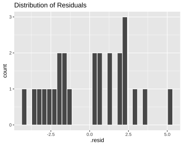
```

![](L4_DOE_files/figure-html/unnamed-chunk-5-1.png)

]

.pull-right[

```r
ggplot(residdf, 
       aes(sample=.resid))+
  stat_qq() + stat_qq_line()+labs(x="Theoretical Quantiles", y="Sample Quantiles")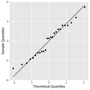
```

![](L4_DOE_files/figure-html/unnamed-chunk-6-1.png)

]

---

# The normality assumption (cont.)

```r
shapiro.test(residdf$.resid)
```

```

Shapiro-Wilk normality test

data:  residdf$.resid
W = 0.96073, p-value = 0.4291
```

---

# Plot of residuals in time sequence

This is helpful in detecting **correlation between residuals**. This is useful to check the validity of the independence assumption on the errors.

```r
residdf$Time <- 1:25
residdf
```

```
# A tibble: 25 × 9
 value Treatment .fitted .resid .hat .sigma .cooksd .std.resid Time
 <dbl> <chr> <dbl> <dbl> <dbl> <dbl> <dbl> <dbl> <int>
 1 8 A 9.80 -1.80 0.200 2.78 0.0268 -0.732 1
 2 11 B 15.2 -4.20 0.200 2.61 0.146 -1.71 2
 3 14 C 17.6 -3.60 0.2 2.67 0.107 -1.46 3
 4 20 D 21.6 -1.60 0.2 2.79 0.0212 -0.651 4
 5 8 E 11.4 -3.40 0.2 2.68 0.0956 -1.38 5
 6 8 A 9.80 -1.80 0.2 2.78 0.0268 -0.732 6
 7 17 B 15.2 1.80 0.2 2.78 0.0268 0.732 7
 8 16 C 17.6 -1.60 0.2 2.79 0.0212 -0.651 8
 9 24 D 21.6 2.40 0.2 2.75 0.0476 0.976 9
10 10 E 11.4 -1.40 0.2 2.80 0.0162 -0.569 10
# … with 15 more rows
```

---

# Plot of residuals in time sequence (cont.)

```r
ggplot(data=residdf, aes(x=Time, y=.resid)) + geom_point()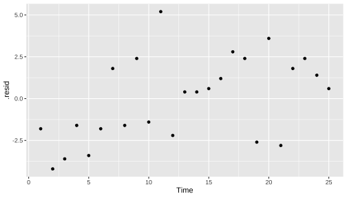
```

![](L4_DOE_files/figure-html/unnamed-chunk-9-1.png)

Residuals should be structureless. Residuals should not contain any obvious patterns.

---

# Plot of residuals versus fitted values

- To check the assumption of constant variance

- Residuals should be structureless. Residuals should not contain any obvious patterns

```r
ggplot(data=residdf, aes(x=.fitted, y=.resid)) + geom_point()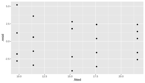
```

![](L4_DOE_files/figure-html/unnamed-chunk-10-1.png)

---

# Statistical Tests for Equality of Variance

Bartlett's test

`$H_0: \sigma^2_1 = \sigma^2_2 = \sigma^2_3 = \sigma^2_4 = \sigma^2_5$`

`$H_1: \text{above not true for at least one } \sigma^2_i$`

```r
bartlett.test(value ~Treatment, residdf)
```

```

Bartlett test of homogeneity of variances

data:  value by Treatment
Bartlett's K-squared = 0.84527, df = 4, p-value = 0.9323
```

Bartlett's test is very sensitive to the assumption of normality. Hence, when the normality assumption is violated Bartlett's test should not be used.

---

Your turn: Bartlett's test

Test statistics:

Distribution of test statistics under the null hypothesis:

---

## ANOVA

```r
one.way <- aov(value ~ Treatment, data = df)
summary(one.way)
```

---

### Comparison among treatment means: multiple comparison

.pull-left[

```r
TukeyHSD(one.way,  "Treatment")
```

```
  Tukey multiple comparisons of means
    95% family-wise confidence level

Fit: aov(formula = value ~ Treatment, data = df)

$Treatment
     diff         lwr        upr     p adj
B-A   5.4   0.1963648 10.6036352 0.0396033
C-A   7.8   2.5963648 13.0036352 0.0018847
D-A  11.8   6.5963648 17.0036352 0.0000122
E-A   1.6  -3.6036352  6.8036352 0.8857969
C-B   2.4  -2.8036352  7.6036352 0.6466099
D-B   6.4   1.1963648 11.6036352 0.0114841
E-B  -3.8  -9.0036352  1.4036352 0.2254122
D-C   4.0  -1.2036352  9.2036352 0.1858647
E-C  -6.2 -11.4036352 -0.9963648 0.0147894
E-D -10.2 -15.4036352 -4.9963648 0.0000863
```

]

.pull-right[

```r
plot(TukeyHSD(one.way,  "Treatment"))
```

![](L4_DOE_files/figure-html/unnamed-chunk-14-1.png)

]

---

.pull-left[

```r
plot(TukeyHSD(one.way,  "Treatment"))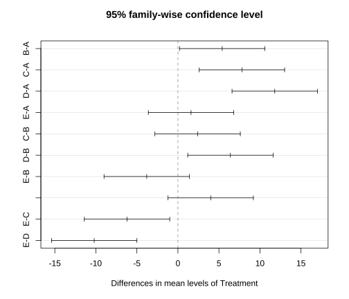
```

![](L4_DOE_files/figure-html/unnamed-chunk-15-1.png)

]

.pull-right[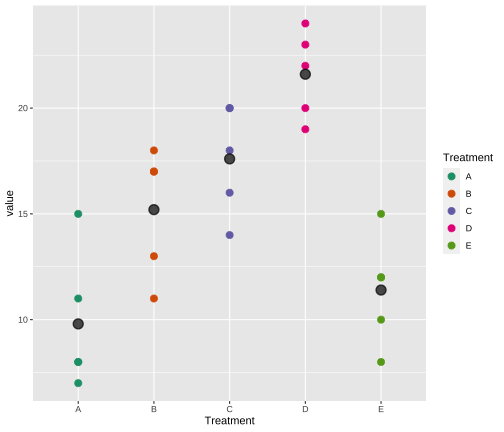
![](L4_DOE_files/figure-html/unnamed-chunk-16-1.png)

]

---

# Acknowledgement

Some of the slide content is based on

Montgomery, D. C. (2017). Design and analysis of experiments. John wiley & sons.