STA 225 2.0 Design and Analysis of Experiments

class: center, middle, inverse, title-slide

# STA 225 2.0 Design and Analysis of Experiments
## Lecture 11-12
### Dr Thiyanga S. Talagala
### 2022-03-08/ 2022-03-25

---

<style>

.center2 {
  margin: 0;
  position: absolute;
  top: 50%;
  left: 50%;
  -ms-transform: translate(-50%, -50%);
  transform: translate(-50%, -50%);
}

</style>

## Factorial Design

- CRD, RCBD, LSD: deal with one factor, hence we called them "simple experiments".

- Useful in experimental situations which involve the study of the effect of two or more factors.

- **Factorial**: the effect of several factors are studied simultaneously

- Treatments: All combinations of the different factor levels

---

## Main effect

- Change in response produced by a change in the level of the factor

.pull-left[
**In-class**

]

.pull-right[

Figure: A factorial experiment without interaction

]

---

## Interaction effect

.pull-left[

**In-class**

]

.pull-right[

Figure: A factorial experiment with interaction

]

---

## The two-factor factorial design

**Life (in hours) Data for the Battery Design Example** (Montgomery, 2004)

```r
library(tidyverse)
material_type <- factor(rep(1:3, each=12))
temperature <- factor(rep(c(15, 70, 125), each=4, times = 3))
life <- c(130, 155, 74, 180, 34, 40, 80, 75, 20, 70, 82, 58, 150, 188, 159, 126, 136, 122, 106, 115, 25, 70, 58, 45, 138, 110, 168, 160, 174, 120, 150, 139, 96, 104, 82, 60)
data <- tibble(material = material_type,
               temperature = temperature,
               life = life)
data
```

```
# A tibble: 36 × 3
   material temperature  life
   <fct>    <fct>       <dbl>
 1 1        15            130
 2 1        15            155
 3 1        15             74
 4 1        15            180
 5 1        70             34
 6 1        70             40
 7 1        70             80
 8 1        70             75
 9 1        125            20
10 1        125            70
# … with 26 more rows
```

---

## Data arrangement

In-class

---

# Possible questions

- What effect do material type and temperature have on the life of the battery?

- Robust product design: Is there a choice of material that would give uniformly long life regardless of temperature (material that is not greatly affected by temperature)?

---

## General arrangement for a two-factorial factor design

---

## The effect model

> In class

`$$y_{ijk} = \mu + \tau_i + \beta_j + (\tau \beta)_{ij} + \epsilon_{ijk}$$`
Introduce all terms and write down the assumptions of the error term
---

## The mean model

> In class

`$$y_{ijk} = \mu_{ij} + \epsilon_{ijk}$$`
Introduce all terms and write down the assumptions of the error term

---
## Testing hypotheses

1. equality of row treatment effect

H0: `$\tau_1=\tau_2=...=\tau_a=0$`

H1: at least one `$\tau_i \neq 0$`

2. equality of column treatment effect

H0: `$\beta_1=\beta_2=...=\beta_b=0$`

H1: at least one `$\beta_i \neq 0$`

3. equality of row and column treatments interact

H0: `$(\tau\beta)_{ij}=0$` for all `$i, j$`

H1: at least one `$(\tau\beta)_{ij} \neq 0$`

---

## Total of observations and grand mean

.pull-left[

### Total

`$$y_{...} = \sum_{i=1}^a\sum_{j=1}^b\sum_{k=1}^n y_{ijk}$$`

]

.pull-right[

### Mean

`$$\bar{y}_{...} = \frac{y_{...}}{abn}$$`

]

---

.pull-left[
### Total of observations under the `$i$`th level of factor A

`$$y_{i..}=\sum_{j=1}^b\sum_{k=1}^n y_{ijk}$$`

]

.pull-right[

### Mean

`$$\bar{y}_{i..} = \frac{y_{i..}}{bn}$$`

]

---

.pull-left[
### Total of observations under the `$j$`th level of factor B

`$$y_{.j.}= \sum_{i=1}^a\sum_{k=1}^n y_{ijk}$$`

]

.pull-right[

### Mean

`$$\bar{y}_{.j.} = \frac{y_{.j.}}{an}$$`

]

---

.pull-left[

### Total of all observations in the `$ij$`th cell

`$$y_{ij.}= \sum_{k=1}^n y_{ijk}$$`

]

.pull-right[

### Mean

`$$\bar{y}_{ij.} = \frac{y_{ij.}}{n}$$`

]

---
## Total sum of squares

`$$\sum_{i=1}^a\sum_{j=1}^b\sum_{k=1}^n (y_{ijk} - \bar{y}_{...})^2=\sum_{i=1}^a\sum_{j=1}^b\sum_{k=1}^n[(\bar{y}_{i..}-\bar{y}_{...}) + (\bar{y}_{.j.} - \bar{y}_{...}) + (\bar{y}_{ij.} - \bar{y}_{i..} - \bar{y}_{.j.}+\bar{y}_{...}) + (y_{ijk} - \bar{y}_{ij.})]^2$$`

Show that

`$$SS_T = SS_A + SS_B + SS_{AB} + SS_{E}$$`

---

## Degrees of freedom associated with sum of squares

> A : a-1

> B: b-1

> AB interaction: (a-1)(b-1)

> Error: ab(n-1)

> Total: abn-1

---

## ANOVA table

> In class

---
## EDA

.pull-left[

```r
ggplot(data, aes(x=material, y=life, col=material)) + geom_boxplot() + geom_jitter()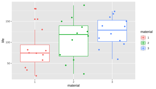
```

![](L8_DOE_files/figure-html/unnamed-chunk-2-1.png)

]

.pull-right[

```r
ggplot(data, aes(x=temperature, y=life, col=temperature)) + geom_boxplot() + geom_jitter()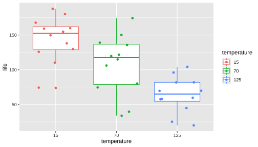
```

![](L8_DOE_files/figure-html/unnamed-chunk-3-1.png)

]

---

```r
data %>% group_by(temperature) %>%
  summarize(mean = mean(life), sd=sd(life))
```

```
## # A tibble: 3 × 3
##   temperature  mean    sd
##   <fct>       <dbl> <dbl>
## 1 15          145.   31.7
## 2 70          108.   42.9
## 3 125          64.2  25.7
```

```r
data %>% group_by(material) %>%
  summarize(mean = mean(life), sd=sd(life))
```

```
## # A tibble: 3 × 3
##   material  mean    sd
##   <fct>    <dbl> <dbl>
## 1 1         83.2  48.6
## 2 2        108.   49.5
## 3 3        125.   35.8
```

---
## ANOVA

```r
head(data)
```

```
## # A tibble: 6 × 3
##   material temperature  life
##   <fct>    <fct>       <dbl>
## 1 1        15            130
## 2 1        15            155
## 3 1        15             74
## 4 1        15            180
## 5 1        70             34
## 6 1        70             40
```

```r
fit <- lm(life ~ temperature + material + temperature * material, data=data)
```

---

## ANOVA

```r
anova(fit)
```

```
## Analysis of Variance Table
## 
## Response: life
##                      Df Sum Sq Mean Sq F value    Pr(>F)    
## temperature           2  39119 19559.4 28.9677 1.909e-07 ***
## material              2  10684  5341.9  7.9114  0.001976 ** 
## temperature:material  4   9614  2403.4  3.5595  0.018611 *  
## Residuals            27  18231   675.2                      
## ---
## Signif. codes:  0 '***' 0.001 '**' 0.01 '*' 0.05 '.' 0.1 ' ' 1
```

---
## Manual computation

Total sum of squares

`$$SS_T = \sum_{i=1}^{a}\sum_{j=1}^b\sum_{k=1}^ny^2_{ijk} - \frac{y^2_{...}}{abn}$$`

Sum of squares for the main effects

`$$SS_A = \frac{1}{bn}\sum_{i=1}^{a}y^2_{i..} - \frac{y^2_{...}}{abn}$$`

`$$SS_B = \frac{1}{an}\sum_{i=1}^{b}y^2_{.j.} - \frac{y^2_{...}}{abn}$$`

---

Sum of squares between the *ab* cell totals

`$$SS_{Subtotals} = \frac{1}{n}\sum_{i=1}^{a}\sum_{j=1}^by^2_{ij.} - \frac{y^2_{...}}{abn}$$`

`$$SS_{AB} = SS_{Subtotals} - SS_A - SS_B$$`

`$$SS_E = SS_T - SS_{Subtotals}$$`

---

## Model Adequacy Checking

```r
resid_fit <- broom::augment(fit)
resid_fit
```

```
## # A tibble: 36 × 9
##     life temperature material .fitted .resid  .hat .sigma .cooksd .std.resid
##    <dbl> <fct>       <fct>      <dbl>  <dbl> <dbl>  <dbl>   <dbl>      <dbl>
##  1   130 15          1          135.   -4.75 0.250   26.5 0.00165     -0.211
##  2   155 15          1          135.   20.3  0.250   26.1 0.0300       0.900
##  3    74 15          1          135.  -60.7  0.250   22.6 0.270       -2.70 
##  4   180 15          1          135.   45.3  0.250   24.4 0.150        2.01 
##  5    34 70          1           57.2 -23.2  0.25    26.0 0.0395      -1.03 
##  6    40 70          1           57.2 -17.2  0.25    26.2 0.0218      -0.767
##  7    80 70          1           57.2  22.8  0.25    26.0 0.0379       1.01 
##  8    75 70          1           57.2  17.8  0.25    26.2 0.0230       0.789
##  9    20 125         1           57.5 -37.5  0.25    25.1 0.103       -1.67 
## 10    70 125         1           57.5  12.5  0.25    26.3 0.0114       0.555
## # … with 26 more rows
```

---

## Assumption

We assume that the error terms `$\epsilon_{ijk}$` are normally and independently distributed with constant variance `$\sigma^2$`.

---

## Normality plot of residuals

.pull-left[

```r
ggplot(resid_fit, 
       aes(sample=.resid))+
  stat_qq() + stat_qq_line()+labs(x="Theoretical Quantiles", y="Sample Quantiles")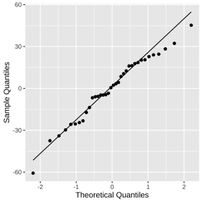
```

![](L8_DOE_files/figure-html/unnamed-chunk-8-1.png)

]

.pull-right[

```r
shapiro.test(resid_fit$.resid)
```

```
## 
## 	Shapiro-Wilk normality test
## 
## data:  resid_fit$.resid
## W = 0.97606, p-value = 0.6117
```

]

---

## Residuals vs Fitted Values

```r
ggplot(resid_fit, aes(x=.fitted, y=.resid)) + geom_point()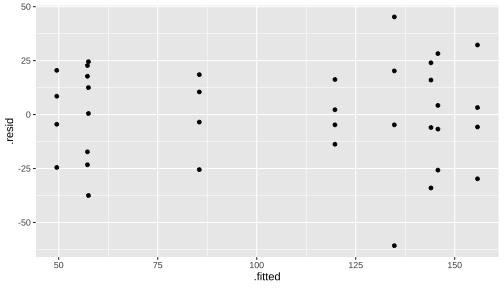
```

![](L8_DOE_files/figure-html/unnamed-chunk-10-1.png)

---

## Plot of residuals vs material type

```r
ggplot(resid_fit, aes(x=material, y=.resid)) + geom_point()
```

![](L8_DOE_files/figure-html/unnamed-chunk-11-1.png)

---

## Plot of residuals vs temperature

```r
ggplot(resid_fit, aes(x=temperature, y=.resid)) + geom_point()
```

![](L8_DOE_files/figure-html/unnamed-chunk-12-1.png)

---

## ANOVA table interpretation

```r
anovatab <- anova(fit)
anovatab
```

---

### Graph of average responses at each treatment combination

```r
average_responses <- data %>% group_by(temperature, material) %>% summarize(mean=mean(life))
average_responses 
```

```
## # A tibble: 9 × 3
## # Groups:   temperature [3]
##   temperature material  mean
##   <fct>       <fct>    <dbl>
## 1 15          1        135. 
## 2 15          2        156. 
## 3 15          3        144  
## 4 70          1         57.2
## 5 70          2        120. 
## 6 70          3        146. 
## 7 125         1         57.5
## 8 125         2         49.5
## 9 125         3         85.5
```

---

### Graph of average responses at each treatment combination

```r
ggplot(average_responses, aes(x=temperature, y=mean, group=material, col=material)) + geom_point() + geom_path() 
```

![](L8_DOE_files/figure-html/unnamed-chunk-15-1.png)

---

## Interpretation

> If there is a significant interaction between factor A and factor B

- Omit the tests for main effects when interaction is present.

- Reason: The interaction indicates that the relationship between the levels of factor A vary with the levels of factor B

---

## Interpretation

> If there is no significant interaction

- Then the tests for main effects easily interpreted

- For example we can conclude that there are significant differences between at least two levels of factor A. Further, these differences should be similar at each level of factor B. Then you can use multiple comparisons to determine which levels of factor A are significantly different.

---

## Multiple comparisons: when interaction effect is present

- Perform the multiple comparisons on the "ab" treatments (cell means).

- Alternatively, a user might want to compare the levels of factor A for a specified levels of factor B

---

## Multiple comparisons

```r
aov.out <- aov(life ~ material * temperature, data=data)
aov.out
```

```
Call:
   aov(formula = life ~ material * temperature, data = data)

Terms:
                material temperature material:temperature Residuals
Sum of Squares  10683.72    39118.72              9613.78  18230.75
Deg. of Freedom        2           2                    4        27

Residual standard error: 25.98486
Estimated effects may be unbalanced
```

---

```r
results <- TukeyHSD(aov.out)
results
```

```
##   Tukey multiple comparisons of means
##     95% family-wise confidence level
## 
## Fit: aov(formula = life ~ material * temperature, data = data)
## 
## $material
##         diff       lwr      upr     p adj
## 2-1 25.16667 -1.135677 51.46901 0.0627571
## 3-1 41.91667 15.614323 68.21901 0.0014162
## 3-2 16.75000 -9.552344 43.05234 0.2717815
## 
## $temperature
##             diff        lwr       upr     p adj
## 70-15  -37.25000  -63.55234 -10.94766 0.0043788
## 125-15 -80.66667 -106.96901 -54.36432 0.0000001
## 125-70 -43.41667  -69.71901 -17.11432 0.0009787
## 
## $`material:temperature`
##                diff         lwr        upr     p adj
## 2:15-1:15     21.00  -40.823184  82.823184 0.9616404
## 3:15-1:15      9.25  -52.573184  71.073184 0.9998527
## 1:70-1:15    -77.50 -139.323184 -15.676816 0.0065212
## 2:70-1:15    -15.00  -76.823184  46.823184 0.9953182
## 3:70-1:15     11.00  -50.823184  72.823184 0.9994703
## 1:125-1:15   -77.25 -139.073184 -15.426816 0.0067471
## 2:125-1:15   -85.25 -147.073184 -23.426816 0.0022351
## 3:125-1:15   -49.25 -111.073184  12.573184 0.2016535
## 3:15-2:15    -11.75  -73.573184  50.073184 0.9991463
## 1:70-2:15    -98.50 -160.323184 -36.676816 0.0003449
## 2:70-2:15    -36.00  -97.823184  25.823184 0.5819453
## 3:70-2:15    -10.00  -71.823184  51.823184 0.9997369
## 1:125-2:15   -98.25 -160.073184 -36.426816 0.0003574
## 2:125-2:15  -106.25 -168.073184 -44.426816 0.0001152
## 3:125-2:15   -70.25 -132.073184  -8.426816 0.0172076
## 1:70-3:15    -86.75 -148.573184 -24.926816 0.0018119
## 2:70-3:15    -24.25  -86.073184  37.573184 0.9165175
## 3:70-3:15      1.75  -60.073184  63.573184 1.0000000
## 1:125-3:15   -86.50 -148.323184 -24.676816 0.0018765
## 2:125-3:15   -94.50 -156.323184 -32.676816 0.0006078
## 3:125-3:15   -58.50 -120.323184   3.323184 0.0742711
## 2:70-1:70     62.50    0.676816 124.323184 0.0460388
## 3:70-1:70     88.50   26.676816 150.323184 0.0014173
## 1:125-1:70     0.25  -61.573184  62.073184 1.0000000
## 2:125-1:70    -7.75  -69.573184  54.073184 0.9999614
## 3:125-1:70    28.25  -33.573184  90.073184 0.8281938
## 3:70-2:70     26.00  -35.823184  87.823184 0.8822881
## 1:125-2:70   -62.25 -124.073184  -0.426816 0.0474675
## 2:125-2:70   -70.25 -132.073184  -8.426816 0.0172076
## 3:125-2:70   -34.25  -96.073184  27.573184 0.6420441
## 1:125-3:70   -88.25 -150.073184 -26.426816 0.0014679
## 2:125-3:70   -96.25 -158.073184 -34.426816 0.0004744
## 3:125-3:70   -60.25 -122.073184   1.573184 0.0604247
## 2:125-1:125   -8.00  -69.823184  53.823184 0.9999508
## 3:125-1:125   28.00  -33.823184  89.823184 0.8347331
## 3:125-2:125   36.00  -25.823184  97.823184 0.5819453
```

---

```r
dim(results$`material:temperature`)
```

```
## [1] 36  4
```
---

```r
results$`material:temperature`[1:18, ]
```

```
##               diff        lwr        upr        p adj
## 2:15-1:15    21.00  -40.82318  82.823184 0.9616403972
## 3:15-1:15     9.25  -52.57318  71.073184 0.9998527390
## 1:70-1:15   -77.50 -139.32318 -15.676816 0.0065212148
## 2:70-1:15   -15.00  -76.82318  46.823184 0.9953181940
## 3:70-1:15    11.00  -50.82318  72.823184 0.9994702697
## 1:125-1:15  -77.25 -139.07318 -15.426816 0.0067471137
## 2:125-1:15  -85.25 -147.07318 -23.426816 0.0022350689
## 3:125-1:15  -49.25 -111.07318  12.573184 0.2016535112
## 3:15-2:15   -11.75  -73.57318  50.073184 0.9991463221
## 1:70-2:15   -98.50 -160.32318 -36.676816 0.0003449173
## 2:70-2:15   -36.00  -97.82318  25.823184 0.5819453144
## 3:70-2:15   -10.00  -71.82318  51.823184 0.9997369049
## 1:125-2:15  -98.25 -160.07318 -36.426816 0.0003573540
## 2:125-2:15 -106.25 -168.07318 -44.426816 0.0001151507
## 3:125-2:15  -70.25 -132.07318  -8.426816 0.0172076171
## 1:70-3:15   -86.75 -148.57318 -24.926816 0.0018118976
## 2:70-3:15   -24.25  -86.07318  37.573184 0.9165174549
## 3:70-3:15     1.75  -60.07318  63.573184 0.9999999997
```

---

```r
results$`material:temperature`[19:30, ]
```

```
##              diff         lwr        upr        p adj
## 1:125-3:15 -86.50 -148.323184 -24.676816 0.0018764896
## 2:125-3:15 -94.50 -156.323184 -32.676816 0.0006077696
## 3:125-3:15 -58.50 -120.323184   3.323184 0.0742710994
## 2:70-1:70   62.50    0.676816 124.323184 0.0460387808
## 3:70-1:70   88.50   26.676816 150.323184 0.0014172574
## 1:125-1:70   0.25  -61.573184  62.073184 1.0000000000
## 2:125-1:70  -7.75  -69.573184  54.073184 0.9999613693
## 3:125-1:70  28.25  -33.573184  90.073184 0.8281938115
## 3:70-2:70   26.00  -35.823184  87.823184 0.8822881387
## 1:125-2:70 -62.25 -124.073184  -0.426816 0.0474674659
## 2:125-2:70 -70.25 -132.073184  -8.426816 0.0172076171
## 3:125-2:70 -34.25  -96.073184  27.573184 0.6420440941
```

The analysis indicates that **at the temperature level 70** there is no significant difference between the mean battery life for material type 2 and type 3. However, there is a significant difference between mean battery life for material types between 2 and 1. Furthermore, there is a significant difference between mean battery life for material types 3 and 1. Mean battery life for material type 1 is significantly lower in comparison to both material type 2 and 3

---

## Manual calculations

Studentized range statistic

`$$q = \frac{\bar{y}_{max}-\bar{y}_{min}}{\sqrt{MS_E/n}}$$`

`$$T_\alpha = q_\alpha(a, f) \sqrt{\frac{MS_E}{n}}$$`
`$a$` - treatments

`$f$` - number of degrees of freedom associated with `$MS_E$`

---
Three material (a=3) type at temperature 70

`$$T_{0.05} = q_{0.05}(3, 27) \sqrt{\frac{675.21}{4}} = 45.47$$`

.pull-left[
`$$\bar{y}_{12.} = 57.25$$`
`$$\bar{y}_{22.} = 119.75$$`

`$$\bar{y}_{32.} = 145.75$$`

]

.pull-right[

**3 vs 1**: `$145.75 - 57.25 = 88.50 > T_{0.05}$`

**3 vs 2**: `$145.75 - 119.75 = 26.00 < T_{0.05}$`

**2 vs 1**: `$119.75 - 57.25 = 62.50 > T_{0.05}$`

]

---

## Example:

Does the effect of sunlight on plant growth depend on watering frequency?

```
    sunlight  water    growth
1        Low  Daily 11.602699
2        Low  Daily  8.788627
3        Low  Daily  2.837764
4        Low  Daily 10.350109
5        Low  Daily 10.586840
6        Low  Daily 12.593023
7        Low  Daily  2.374750
8        Low  Daily 13.806439
9        Low  Daily 11.880857
10       Low  Daily 11.383926
11       Low  Daily 13.296031
12       Low  Daily  9.811383
13       Low  Daily  6.083509
14       Low  Daily  7.747825
15       Low  Daily 11.848674
16    Medium  Daily 12.278993
17    Medium  Daily  6.422065
18    Medium  Daily 14.956996
19    Medium  Daily 13.302550
20    Medium  Daily  5.539841
21    Medium  Daily 18.543803
22    Medium  Daily  8.814481
23    Medium  Daily 14.133272
24    Medium  Daily 12.973521
25    Medium  Daily  8.668584
26    Medium  Daily 13.666569
27    Medium  Daily 10.272770
28    Medium  Daily  5.935407
29    Medium  Daily 14.202236
30    Medium  Daily  7.311347
31      High  Daily 12.455280
32      High  Daily 12.702102
33      High  Daily 18.179540
34      High  Daily 13.348311
35      High  Daily  9.569833
36      High  Daily 13.940489
37      High  Daily 11.590162
38      High  Daily 11.754965
39      High  Daily 11.656025
40      High  Daily  9.090323
41      High  Daily 11.408538
42      High  Daily 10.225797
43      High  Daily  9.035619
44      High  Daily  7.874920
45      High  Daily 16.295417
46       Low Weekly  5.612127
47       Low Weekly  2.796371
48       Low Weekly  8.092031
49       Low Weekly  7.682207
50       Low Weekly  5.865978
51       Low Weekly 10.495029
52       Low Weekly  2.247268
53       Low Weekly  6.211078
54       Low Weekly  5.735937
55       Low Weekly  8.557471
56       Low Weekly  5.366155
57       Low Weekly  8.859972
58       Low Weekly  8.755086
59       Low Weekly 11.031062
60       Low Weekly  5.549028
61    Medium Weekly 12.671094
62    Medium Weekly 10.833332
63    Medium Weekly 13.519200
64    Medium Weekly 11.796179
65    Medium Weekly  9.522459
66    Medium Weekly  9.019963
67    Medium Weekly  7.088617
68    Medium Weekly 14.981191
69    Medium Weekly  9.987386
70    Medium Weekly  8.765056
71    Medium Weekly  8.949763
72    Medium Weekly 11.021614
73    Medium Weekly 10.969631
74    Medium Weekly  4.817212
75    Medium Weekly  9.056691
76      High Weekly 12.357894
77      High Weekly  9.585223
78      High Weekly  9.322410
79      High Weekly 14.694987
80      High Weekly 10.025044
81      High Weekly  8.795878
82      High Weekly  4.912749
83      High Weekly 12.643520
84      High Weekly  7.615474
85      High Weekly 13.981438
86      High Weekly 12.742762
87      High Weekly  8.238243
88      High Weekly 13.147403
89      High Weekly  9.195736
90      High Weekly 11.110050
91       Low  Daily 11.602699
92       Low  Daily  8.788627
93       Low  Daily  2.837764
94       Low  Daily 10.350109
95       Low  Daily 10.586840
96       Low  Daily 12.593023
97       Low  Daily  2.374750
98       Low  Daily 13.806439
99       Low  Daily 11.880857
100      Low  Daily 11.383926
101      Low  Daily 13.296031
102      Low  Daily  9.811383
103      Low  Daily  6.083509
104      Low  Daily  7.747825
105      Low  Daily 11.848674
106   Medium  Daily 12.278993
107   Medium  Daily  6.422065
108   Medium  Daily 14.956996
109   Medium  Daily 13.302550
110   Medium  Daily  5.539841
111   Medium  Daily 18.543803
112   Medium  Daily  8.814481
113   Medium  Daily 14.133272
114   Medium  Daily 12.973521
115   Medium  Daily  8.668584
116   Medium  Daily 13.666569
117   Medium  Daily 10.272770
118   Medium  Daily  5.935407
119   Medium  Daily 14.202236
120   Medium  Daily  7.311347
121     High  Daily 12.455280
122     High  Daily 12.702102
123     High  Daily 18.179540
124     High  Daily 13.348311
125     High  Daily  9.569833
126     High  Daily 13.940489
127     High  Daily 11.590162
128     High  Daily 11.754965
129     High  Daily 11.656025
130     High  Daily  9.090323
131     High  Daily 11.408538
132     High  Daily 10.225797
133     High  Daily  9.035619
134     High  Daily  7.874920
135     High  Daily 16.295417
136      Low Weekly  5.612127
137      Low Weekly  2.796371
138      Low Weekly  8.092031
139      Low Weekly  7.682207
140      Low Weekly  5.865978
141      Low Weekly 10.495029
142      Low Weekly  2.247268
143      Low Weekly  6.211078
144      Low Weekly  5.735937
145      Low Weekly  8.557471
146      Low Weekly  5.366155
147      Low Weekly  8.859972
148      Low Weekly  8.755086
149      Low Weekly 11.031062
150      Low Weekly  5.549028
151   Medium Weekly 12.671094
152   Medium Weekly 10.833332
153   Medium Weekly 13.519200
154   Medium Weekly 11.796179
155   Medium Weekly  9.522459
156   Medium Weekly  9.019963
157   Medium Weekly  7.088617
158   Medium Weekly 14.981191
159   Medium Weekly  9.987386
160   Medium Weekly  8.765056
161   Medium Weekly  8.949763
162   Medium Weekly 11.021614
163   Medium Weekly 10.969631
164   Medium Weekly  4.817212
165   Medium Weekly  9.056691
166     High Weekly 12.357894
167     High Weekly  9.585223
168     High Weekly  9.322410
169     High Weekly 14.694987
170     High Weekly 10.025044
171     High Weekly  8.795878
172     High Weekly  4.912749
173     High Weekly 12.643520
174     High Weekly  7.615474
175     High Weekly 13.981438
176     High Weekly 12.742762
177     High Weekly  8.238243
178     High Weekly 13.147403
179     High Weekly  9.195736
180     High Weekly 11.110050
```

---

## Descriptive Statistics

```r
summary(df)
```

```
   sunlight     water        growth      
 High  :60   Daily :90   Min.   : 2.247  
 Low   :60   Weekly:90   1st Qu.: 8.092  
 Medium:60               Median :10.125  
                         Mean   :10.060  
                         3rd Qu.:12.593  
                         Max.   :18.544  
```

---

```r
t1 <- df %>% group_by(sunlight, water) %>% summarize(mean=mean(growth))
```

```
## `summarise()` has grouped output by 'sunlight'. You can override using the
## `.groups` argument.
```

```r
t1
```

```
## # A tibble: 6 × 3
## # Groups:   sunlight [3]
##   sunlight water   mean
##   <fct>    <fct>  <dbl>
## 1 High     Daily  11.9 
## 2 High     Weekly 10.6 
## 3 Low      Daily   9.67
## 4 Low      Weekly  6.86
## 5 Medium   Daily  11.1 
## 6 Medium   Weekly 10.2
```

Draw the interaction plot and comment on it.

---

```r
ggplot(t1, aes(x=sunlight, y=mean, group=water, col=water)) + geom_point() + geom_path()
```

![](L8_DOE_files/figure-html/unnamed-chunk-24-1.png)

---

```r
fit2 <- lm(growth ~ sunlight + water + sunlight*water, data=df)
anova(fit2)
```

```
## Analysis of Variance Table
## 
## Response: growth
##                 Df  Sum Sq Mean Sq F value    Pr(>F)    
## sunlight         2  301.13 150.564 16.9591 1.867e-07 ***
## water            1  131.47 131.472 14.8086 0.0001669 ***
## sunlight:water   2   28.73  14.363  1.6178 0.2013041    
## Residuals      174 1544.79   8.878                      
## ---
## Signif. codes:  0 '***' 0.001 '**' 0.01 '*' 0.05 '.' 0.1 ' ' 1
```

---

## Compute residuals and fitted values

```r
t2 <- broom::augment(fit2)
t2
```

```
## # A tibble: 180 × 9
##    growth sunlight water .fitted .resid   .hat .sigma  .cooksd .std.resid
##     <dbl> <fct>    <fct>   <dbl>  <dbl>  <dbl>  <dbl>    <dbl>      <dbl>
##  1  11.6  Low      Daily    9.67  1.94  0.0333   2.98 0.00251       0.661
##  2   8.79 Low      Daily    9.67 -0.878 0.0333   2.99 0.000516     -0.300
##  3   2.84 Low      Daily    9.67 -6.83  0.0333   2.94 0.0312       -2.33 
##  4  10.4  Low      Daily    9.67  0.684 0.0333   2.99 0.000313      0.233
##  5  10.6  Low      Daily    9.67  0.921 0.0333   2.99 0.000568      0.314
##  6  12.6  Low      Daily    9.67  2.93  0.0333   2.98 0.00574       0.999
##  7   2.37 Low      Daily    9.67 -7.29  0.0333   2.93 0.0356       -2.49 
##  8  13.8  Low      Daily    9.67  4.14  0.0333   2.97 0.0115        1.41 
##  9  11.9  Low      Daily    9.67  2.21  0.0333   2.98 0.00328       0.756
## 10  11.4  Low      Daily    9.67  1.72  0.0333   2.99 0.00198       0.586
## # … with 170 more rows
```

---
## Normality plot of residuals

.pull-left[

```r
ggplot(t2, 
       aes(sample=.resid))+
  stat_qq() + stat_qq_line()+labs(x="Theoretical Quantiles", y="Sample Quantiles")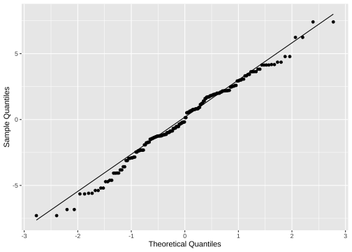
```

![](L8_DOE_files/figure-html/unnamed-chunk-27-1.png)

]

.pull-left[

```r
shapiro.test(t2$.resid)
```

```
## 
## 	Shapiro-Wilk normality test
## 
## data:  t2$.resid
## W = 0.98796, p-value = 0.1292
```

]

---

## Residuals vs Fitted

```r
ggplot(t2, aes(x=.fitted, y=.resid)) + geom_point()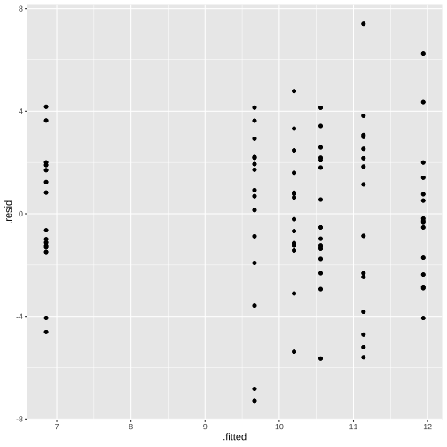
```

![](L8_DOE_files/figure-html/unnamed-chunk-29-1.png)

---

## Plot of residuals vs water level

```r
ggplot(t2, aes(x=water, y=.resid)) + geom_point()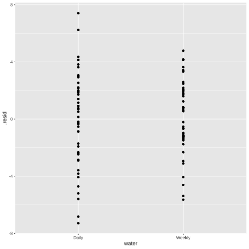
```

![](L8_DOE_files/figure-html/unnamed-chunk-30-1.png)

---
## Plot of residuals vs sunlight

```r
ggplot(t2, aes(x=sunlight, y=.resid)) + geom_point()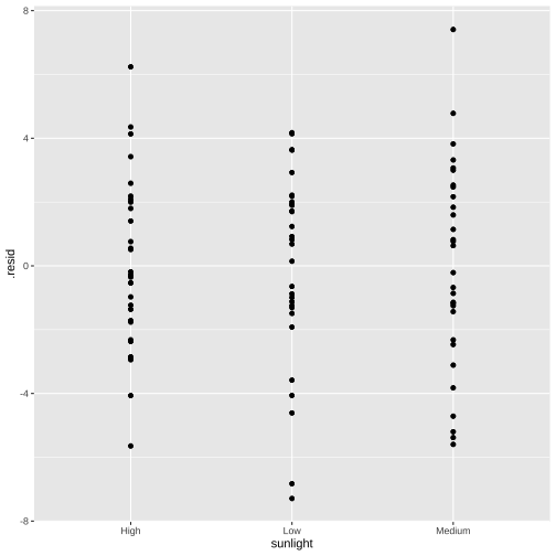
```

![](L8_DOE_files/figure-html/unnamed-chunk-31-1.png)

---
## Multiple comparison

```r
aov2.out <- aov(growth ~ sunlight * water, data=df)
aov2.out
```

```
## Call:
##    aov(formula = growth ~ sunlight * water, data = df)
## 
## Terms:
##                  sunlight     water sunlight:water Residuals
## Sum of Squares   301.1287  131.4724        28.7260 1544.7911
## Deg. of Freedom         2         1              2       174
## 
## Residual standard error: 2.979616
## Estimated effects may be unbalanced
```
---

## Multiple comparison

```r
TukeyHSD(aov2.out)
```

```
##   Tukey multiple comparisons of means
##     95% family-wise confidence level
## 
## Fit: aov(formula = growth ~ sunlight * water, data = df)
## 
## $sunlight
##                  diff       lwr        upr     p adj
## Low-High    -2.988229 -4.274217 -1.7022417 0.0000004
## Medium-High -0.582477 -1.868464  0.7035105 0.5335055
## Medium-Low   2.405752  1.119765  3.6917396 0.0000508
## 
## $water
##                   diff       lwr        upr     p adj
## Weekly-Daily -1.709272 -2.585936 -0.8326073 0.0001669
## 
## $`sunlight:water`
##                                  diff        lwr         upr     p adj
## Low:Daily-High:Daily       -2.2756575 -4.4926790 -0.05863599 0.0405328
## Medium:Daily-High:Daily    -0.8069924 -3.0240139  1.41002911 0.9005046
## High:Weekly-High:Daily     -1.3839007 -3.6009222  0.83312082 0.4692036
## Low:Weekly-High:Daily      -5.0847015 -7.3017230 -2.86767995 0.0000000
## Medium:Weekly-High:Daily   -1.7418623 -3.9588838  0.47515924 0.2145825
## Medium:Daily-Low:Daily      1.4686651 -0.7483564  3.68568661 0.4001563
## High:Weekly-Low:Daily       0.8917568 -1.3252647  3.10877832 0.8554684
## Low:Weekly-Low:Daily       -2.8090440 -5.0260655 -0.59202244 0.0045847
## Medium:Weekly-Low:Daily     0.5337952 -1.6832263  2.75081674 0.9824391
## High:Weekly-Medium:Daily   -0.5769083 -2.7939298  1.64011322 0.9752292
## Low:Weekly-Medium:Daily    -4.2777091 -6.4947306 -2.06068754 0.0000015
## Medium:Weekly-Medium:Daily -0.9348699 -3.1518914  1.28215164 0.8289908
## Low:Weekly-High:Weekly     -3.7008008 -5.9178223 -1.48377925 0.0000474
## Medium:Weekly-High:Weekly  -0.3579616 -2.5749831  1.85905994 0.9972406
## Medium:Weekly-Low:Weekly    3.3428392  1.1258177  5.55986070 0.0003364
```

---
## Acknowledgement

Content is based on "Design and Analysis of Experiments" by Douglas C. Montgomery